Winning Your Fantasy Football League with Statistics

Fantasy football success isn’t just about knowing which players are good—it’s about understanding the mathematical probabilities that govern player performance. Every touchdown pass, rushing yard, and reception has a probability associated with it, and understanding these probabilities can give you a significant edge over your competition.

At its core, probability is the measure of the likelihood that an event will occur, expressed as a number between 0 and 1 (where 0 indicates impossibility and 1 indicates certainty). In fantasy football, we’re constantly dealing with probabilities: the chance a player will score a touchdown, the probability they’ll reach a certain yardage threshold, or the likelihood they’ll play in a given game.

Let’s start with a simple example. If a running back averages 20 carries per game and has rushed for 100+ yards in 8 of his last 16 games, the empirical probability of him reaching 100 rushing yards in any given game is 8/16 = 0.5 or 50%. This is a basic application of probability theory called empirical probability, which is based on observed data rather than theoretical models.

However, fantasy football probability isn’t this simple. We need to consider multiple factors that affect player performance: opponent strength, weather conditions, injuries, game script, and coaching decisions. A more sophisticated approach involves conditional probability—the probability of an event occurring given that another event has occurred.

For example, what’s the probability that a wide receiver will have a big game if his team is trailing by 14 points in the fourth quarter? Historical data might show that in these situations, receivers have a 70% higher chance of reaching their fantasy point projection. This conditional probability can significantly impact your lineup decisions.

Expected value is another crucial probability concept in fantasy football. Expected value represents the average outcome if an experiment (in this case, a player’s performance) is repeated many times. For a player, expected value might be calculated as:

For instance, if a player has a 30% chance of scoring 20+ fantasy points, a 50% chance of scoring 10-19 points, and a 20% chance of scoring under 10 points, his expected value would be:

This mathematical approach helps you evaluate players more objectively. A player with a high ceiling but low probability of reaching it might have the same expected value as a consistent player with a lower ceiling. Understanding this helps you make better roster decisions based on your league’s scoring format and your strategic approach.

Variance is another important statistical concept in fantasy football. Variance measures how spread out a player’s performance is from their average. A player with high variance might have a great week followed by a terrible week, while a low-variance player performs more consistently. In probability terms, this relates to the standard deviation of a player’s fantasy point distribution.

The mathematical relationship between variance and risk is important for lineup construction. In tournaments or high-stakes leagues, you might want players with high variance (high upside) even if their expected value is slightly lower. In head-to-head matchups, you might prefer low-variance players who are more likely to meet their projections.

Bayesian probability is particularly useful for updating player projections as new information becomes available. For example, if a player has historically averaged 15 fantasy points per game but has started the season with 20+ points in three consecutive games, Bayesian analysis helps you update your probability estimates for his future performance while still considering his historical baseline.

Poisson distribution is a probability model that’s particularly relevant for fantasy football. It’s used to model the number of times an event occurs in a fixed interval of time or space. In fantasy football, it can be used to model the probability of a player scoring a certain number of touchdowns or reaching specific yardage milestones.

For example, if a player averages 0.8 rushing touchdowns per game, the Poisson formula can calculate the probability of him scoring 0, 1, 2, or more touchdowns in any given game:

Understanding these probability concepts helps you make more informed decisions about player selection, trade negotiations, and waiver wire pickups. Rather than relying on gut feelings or media hype, you can use mathematical probability to evaluate which players are most likely to help your team win.

Value Over Replacement Player (VORP) is one of the most powerful statistical concepts borrowed from baseball that has found its way into fantasy football analysis. While not as commonly used in football as in baseball, VORP provides a mathematical framework for evaluating player value that goes beyond simple point totals.

VORP measures how much value a player contributes compared to a baseline “replacement” player—typically defined as a readily available free agent or backup who could be acquired with minimal effort. The mathematical concept behind VORP is subtraction: a player’s value minus the replacement level value.

In fantasy football terms, VORP can be calculated by determining the expected points from your starting lineup and subtracting the expected points from a lineup filled with replacement-level players. This requires establishing what constitutes a replacement-level player at each position, which is where mathematical analysis becomes important.

To calculate positional VORP, you first need to establish replacement levels. In a 12-team league with 1 start per position, the replacement level might be the 12th-best player at each position. In a 10-team league with 2 starts per position (like in many PPR leagues), it might be the 20th-best player.

For example, if the 12th-best quarterback is projected for 200 points and your starting quarterback is projected for 280 points, your quarterback’s VORP is 80 points. If the 12th-best running back is projected for 180 points and your starting running back is projected for 250 points, his VORP is 70 points.

This mathematical approach reveals that the quarterback position might have more value than initially apparent. If the gap between the 1st and 12th quarterbacks is larger than the gap between the 1st and 12th running backs, quarterbacks as a whole are more valuable, and you might adjust your draft strategy accordingly.

VORP calculations become more complex when considering different league formats and scoring systems. In PPR (points per reception) leagues, wide receivers and tight ends become more valuable relative to running backs, which affects replacement levels and VORP calculations. The mathematical principle remains the same, but the inputs change.

Dynamic VORP takes into account the changing nature of replacement levels throughout the season. As players get injured or perform better/worse than expected, replacement levels shift, and so does VORP. This requires regularly updating your calculations, which is where mathematical modeling and data analysis become crucial.

Positional scarcity is another mathematical concept related to VORP. Positions with a steeper drop-off in talent (where the difference between the 1st and 12th best players is large) have higher VORP values on average. This mathematical reality explains why running backs were historically valued so highly in fantasy drafts—the position had significant scarcity.

The mathematical beauty of VORP is that it provides a common unit of measurement (fantasy points) for comparing players across positions. Without VORP, comparing a 300-point quarterback to a 200-point running back is difficult. With VORP, you can determine which player provides more value relative to their position’s replacement level.

VORP also helps with roster construction decisions. If you have two players with similar absolute projections but different VORPs, the player with higher VORP is the better choice. This mathematical approach removes emotion and bias from roster decisions, focusing purely on value creation.

In trade evaluations, VORP provides a mathematical framework for determining fair value. If Player A has a VORP of 100 and Player B has a VORP of 70, you would need to receive additional value to make the trade mathematically beneficial. This objective approach can prevent lopsided trades that favor the other team.

VORP calculations can be extended to consider risk and consistency. A player with a high ceiling but low floor might have the same average VORP as a consistent player, but their VORP distributions would be different. Mathematical tools like standard deviation can help quantify this risk, providing a more complete picture of player value.

Understanding VORP and its mathematical underpinnings helps you make better draft decisions, roster moves, and trade evaluations. It transforms fantasy football from a guessing game into a mathematical exercise in value maximization, giving you a significant edge over competitors who rely on intuition alone.

Data visualization is a powerful mathematical tool for identifying patterns in player performance that raw numbers might obscure. Simple graphs can reveal trends that inform your fantasy football decisions, from draft preparation to weekly lineup optimization.

Line graphs are perhaps the most useful visualization for tracking player performance over time. Plotting a player’s weekly fantasy points throughout a season can reveal patterns like improvement, decline, or consistency. The mathematical concept of slope is particularly important here—a positive slope indicates improvement, while a negative slope suggests decline.

For example, if you plot a rookie wide receiver’s fantasy points over his first eight games and see a consistent upward trend, mathematical projection suggests this trend might continue. The slope of the line gives you a quantitative measure of his rate of improvement, which you can use to estimate future performance.

Moving averages are another mathematical tool for trend identification. A 3-game moving average smooths out weekly variance to reveal underlying performance trends. If a player’s 3-game moving average is consistently increasing, it suggests positive momentum even if individual games show volatility.

Scatter plots are useful for identifying correlations between variables. Plotting a player’s fantasy points against their targets, carries, or snaps played can reveal mathematical relationships. A strong positive correlation between targets and fantasy points for a wide receiver confirms that target share is a key driver of his value.

The correlation coefficient (r) quantifies the strength of these relationships mathematically, ranging from -1 (perfect negative correlation) to +1 (perfect positive correlation). A correlation coefficient of 0.8 between a player’s targets and fantasy points indicates a strong positive relationship, meaning more targets generally lead to more fantasy points.

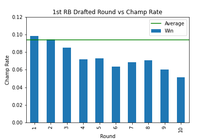
Bar charts can effectively compare players or visualize distributions. A bar chart showing weekly fantasy points for all running backs in your league can help identify which players are consistently performing well. The mathematical concept of central tendency (mean, median) can help you determine what constitutes a “good” week versus an outlier.

Histograms reveal the distribution of player performance, showing how often players achieve different point totals. A normal (bell-shaped) distribution suggests predictable performance, while a skewed distribution indicates that extreme performances (very good or very bad) occur more frequently than expected.

Box plots (box-and-whisker plots) provide a mathematical summary of performance distributions, showing the median, quartiles, and outliers. For fantasy football, box plots can reveal which players are consistent (tight interquartile ranges) versus volatile (wide interquartile ranges with many outliers).

Heat maps are particularly useful for visualizing matchup data. Color-coding opponents by their fantasy points allowed to different positions can quickly reveal favorable and unfavorable matchups. The mathematical principle of data encoding—using color intensity to represent numerical values—makes complex matchup information immediately accessible.

Time series decomposition is a mathematical technique for separating trend, seasonal, and random components of data. In fantasy football, this might reveal that a player consistently performs better in the second half of the season (trend) or that they perform better against divisional opponents (seasonal effect).

Regression analysis can identify mathematical relationships between variables and predict future performance. Simple linear regression might show that a player’s fantasy points can be predicted by their snap count with a certain level of accuracy (R-squared value). This mathematical model can help project performance for players with limited history.

Control charts, borrowed from quality control statistics, can help identify when a player’s performance has significantly changed. If a player’s fantasy points consistently fall outside their historical range of variation, it suggests a real change in their situation rather than random fluctuation.

Percentile rankings provide a mathematical way to compare players within context. If a player’s weekly performance is consistently in the 80th percentile or higher compared to their position, they’re performing well relative to their peers. This mathematical ranking system helps you evaluate players across different statistical categories.

Data visualization tools also help identify when to trust or question projections. If a player’s recent performance trend contradicts their seasonal projections, mathematical analysis of the trend strength can help you determine whether to adjust your expectations.

The mathematical power of data visualization in fantasy football is that it transforms complex numerical relationships into intuitive visual patterns. This makes it easier to process large amounts of information quickly and identify opportunities that your competitors might miss.